Created: January 10, 2019
Last Updated: February 13, 2022

Introduction to Image Matting

A common problem in imaging, which can be defined as the matting problem, is extracting a foreground subject in an image, usually with the goal of placing the foreground subject in a different image Image matting is the process of extracting a foreground subject from an Image.

An ideal matting program would be one that successfully extracts the foreground subject and creates a mask, such that when used to transpose the subject, it would result in a natural image - almost like the foreground subject was there originally.

Matting Terminology

Let the color image $I$ be represented by a 3D tensor of continuous values in the range 0 to 1 - where each dimension of the tensor represents the red, green and blue channels of the image. \ The matting problem involves writing a function matte matte: Image -> (Foreground, alpha) that takes the specified image (3D tensor) and returns the foreground subject(s) $F$ and alpha $\alpha$ channel. \ And it is represented as The Matting Equation

I(x,y) = \alpha(x,y)F(x,y) \space + \space (1 - \alpha(x,y))B(x,y) \space \text{ for each pixel at (x,y)}

or in matrix form as

I = \alpha F + (1 - \alpha)B

Here $I,F,B$ are RGB images (3D Tensor) utilised in the operation - It is also possible to use grayscale images as inputs.

The Alpha $\alpha$ Matte (Channel)

The alpha $\alpha$ channel specifies the degree of variation between the foreground and its background as a matrix of 2D values in the continous domain. \ Producing the alpha matte (mask or matte would be used interchangebly onwards) is different from an image segmentation problem where an alpha matte is produced for each object in the image. Also, compared to image segmentation, the boundaries of the mask contain soft edges (continuous values) between the boundaries of the foreground and background, unlike hard edges (discrete values) in image segmentation. This kind of soft edges are needed because they create a composed image with a natural foreground in it; In high resolution images, the pixels are more pronouced and a hard edge would make the newly composed image look un-natural.

Another case for having continuous values for the matte is that they represent a weighted contribution from objects in the foreground and background. In the optical sense, this could mean that the alpha values contain contribution from the optical rays of the foreground and background objects. \ It is also worth noting that the continuous (fractional) values for the alpha matte can be introduced from motion of the camera or the foreground subject, focal blur induced by the camera aperture and even transparent parts of the foreground subject as a transpared subject would need contributions from its background.

The Foreground $F$ and Background $B$ subject

There are subjective constraints to consider when it comes to image matting. For example, how do we decide what constitutes a foreground or background subject - This descion might vary amongst people. Also there is the question of what if there is no forground subject in the given image too!

For pragmatism, lets assume that there would always be a foreground and background subject in our images, the next question would be deciding on a technique for communicating what constitues a foreground or background.

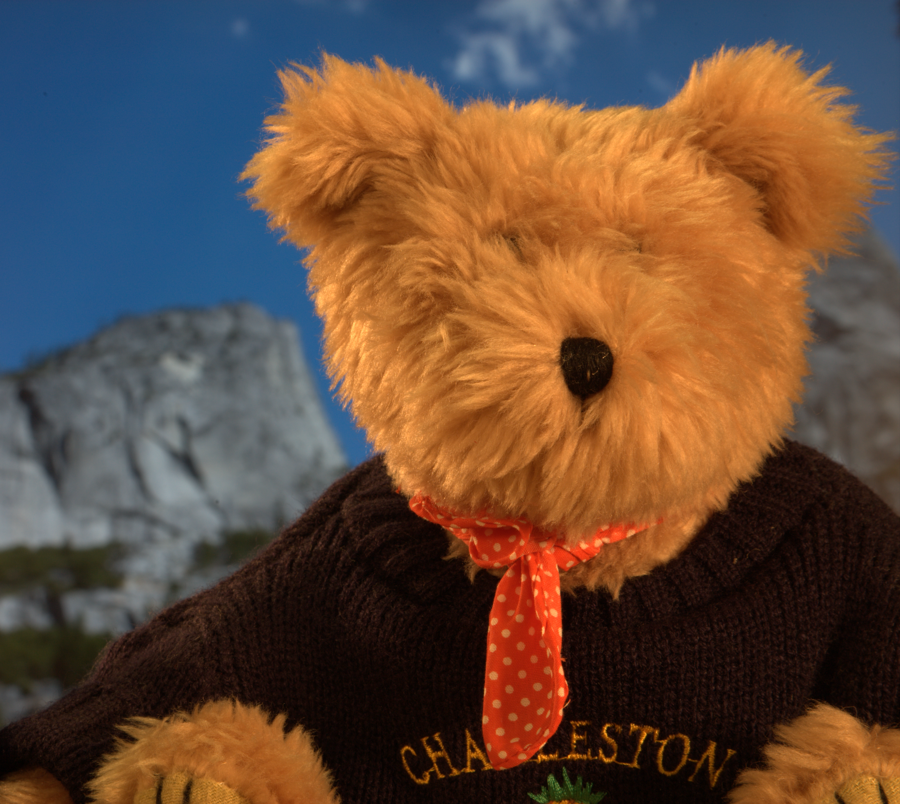
Constant color (Blue/Green) background: Here, the problem is narrowed down with the simple assumption that the background has a particular color. Usually in the Visual Effects (VFX) industry, this can be a blue or green screen background and they are sometimes referred to as the Chromakey.
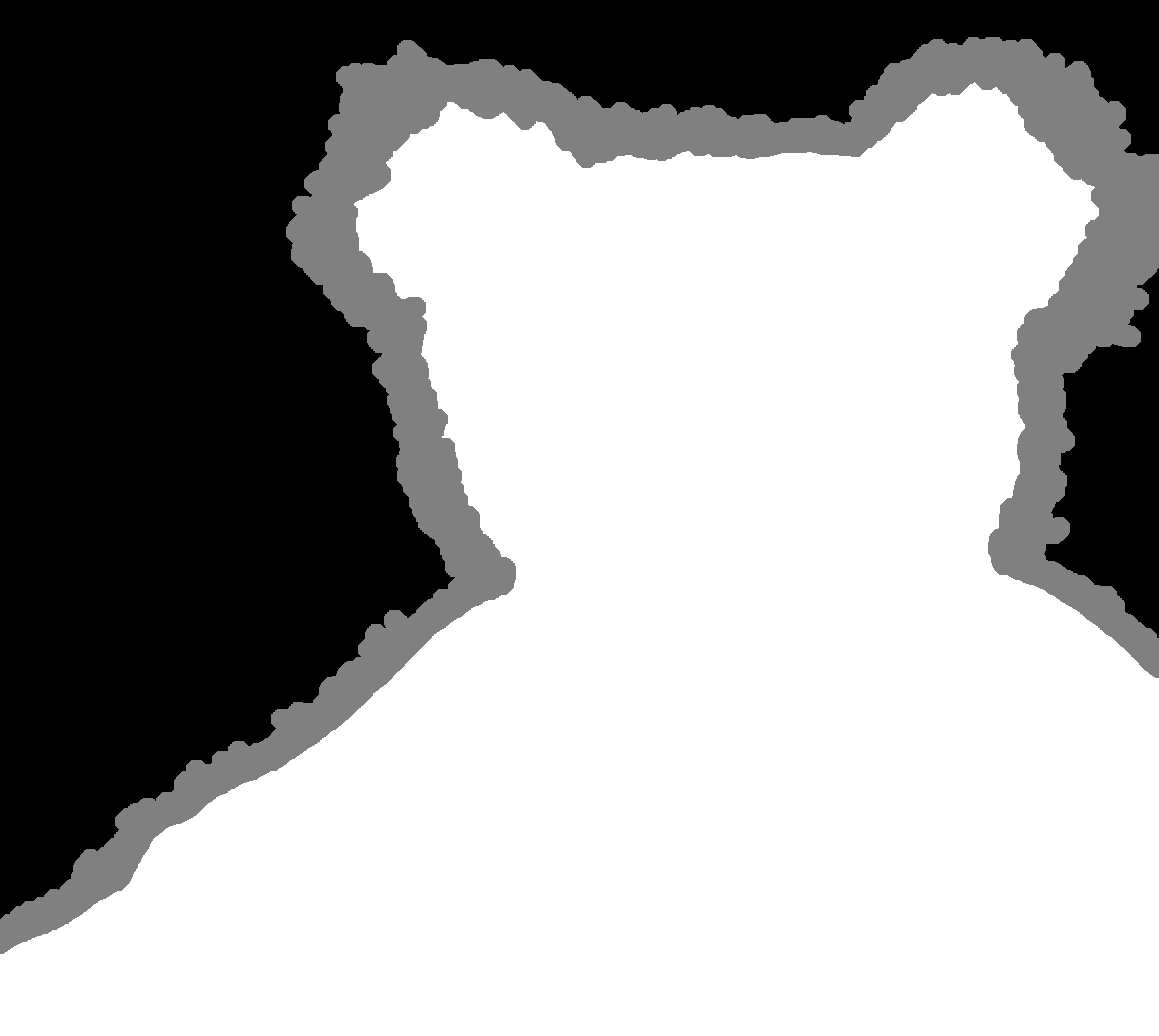
Trimaps: This is useful in complex scenes where the background/foreground is unknown and a pixel is assigned to one of 3 classes. Here an expert user specifies whether a pixel belongs to the foreground $F$ (white pixels in image shown below), background $B$ (black pixels) or an unknown (uncertain) $U$ class (gray pixels). A more extreme version of this is the garbage matte where the user specifies only $B$ and everything else belongs to $U$ .
Scribbles: This is also used in complex scenes but a lot easier to generate. Here the expert user makes sketches that specify a small subset of pixels that are in the foreground and background.

Constant color background — Image with constant color background

Difference Matte

Assuming the user hasn't specified either a colored background (chromakey), a trimap or scribbles - Another source of input is an image called the clean plate . \ The clean plate is an image containing only the background $B$ ; Another image $I$ containing the foreground and background is captured and they can be subtracted to produce a mask as shown below

import numpy as np 
from PIL import Image 

def difference_matte( image, clean_plate ):
    image = image.convert('L') if image.mode == 'RGB' else image 
    clean_plate = clean_plate.convert('L') if clean_plate.mode == 'RGB' else clean_plate 
    image = np.array(image)
    clean_plate = np.array(clean_plate)
    diff = np.abs(image - clean_plate)
    diff[diff >= 125] = 0 # thresholding, needs to be tuned for each image
    return diff

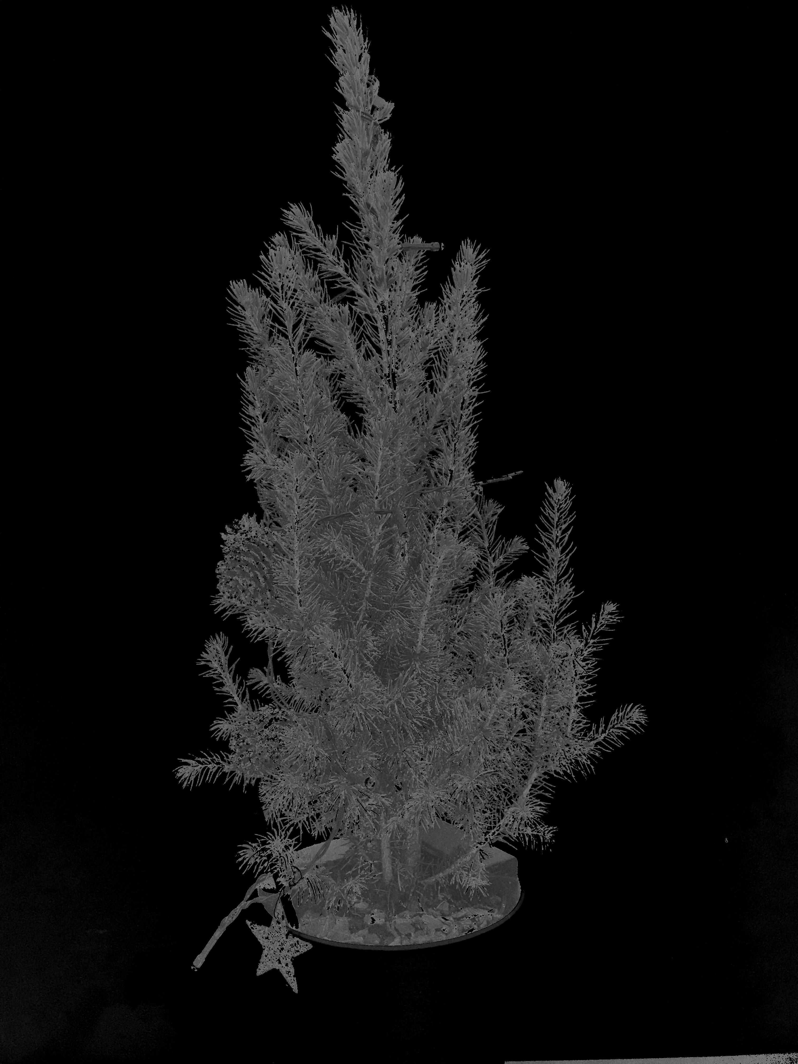
The difference matte simply computes the difference between the image and the clean plate to produce the mask using values greater than a certain threshold, 125 in this case - This is very similar to the thresholding technique used when performing motion detection using the difference between frame sequences. \ This technique is quite error prone compared to the upcoming techniques that would be discussed and it also requires a lot of tweaking to make it work.

For this example, our clean plate is an image of a wall and the input image contains the christmas tree which would be the foreground. One caveat to the difference approach is the little to no room for errors when capturing the clean plate - The surface which the tree rests on is visible in the bottom right of the image and this error is carried over to the calculations of the alpha mask.

def show_difference_matte():
    image = Image.open('difference_image.jpeg')
    clean_plate = Image.open('clean_plate.jpeg')
    alpha = difference_matte(image, clean_plate)
    Image.fromarray(alpha).show()

show_difference_matte()

Due to the threshold of pixels greater than 125, the shadows of the christmas tree and its container are not visible in the alpha mask. While this works for our image, this value would need to be tuned for each respective input image to get the best results.

Blue/Green Screen Matting

These are known as background subtraction in image processing terminology and it involves placing a constant colored background, usually a blue or green chromakey. \ In mathematical terms, lets assume that the foreground subject $F$ has no blue elements to it and the background $B$ is a pure blue one.

F = [r_{F} \space g_{F} \space 0] \\ B = [0 \space 0 \space b_{B}]

Therefore, we can formulate an equation for finding the alpha, $\alpha_{F}$ mask by the matting equation as

I = \alpha_{F} F + (1 - \alpha_{F}) B \\ I = [r_{F} \space g_{F} \space 0] + (1 - \alpha_{F})[0 \space 0 \space b_{B}]

With the assumption that only the background has blue pixels, therefore we can deduce that $r_{F} = r_{I}, g_{F} = g_{I}$ and so on. Therefore,

I = [r_{F} \space g_{F} \space (1 - \alpha_{F})b_{B}]

We can then proceed to solving for $\alpha_{F}$ by remembering that the input image $I = [r_{I} \space g_{I} \space b_{I}]$ and by comparing only the blue channels

b_{I} = (1 - \alpha_{F})b_{B} \\ b_{I} = b_{B} - \alpha_{F}b_{B} \\ \alpha_{F}b_{B} = b_{B} - b_{I} \\ \alpha_{F} = \frac{b_{B} - b_{I}}{b_{B}} \\ \alpha_{F} = (1 - \frac{b_{I}}{b_{B}})

Therefore, the mask $F$ of the foreground, can be written in vector form with the alpha channel as the fourth element as

F = [r_{I} \space g_{I} \space 0 \space (1 - \frac{b_{I}}{b_{B}})], \space \text{ if } b_{B} \neq 0

Vlahos Matting

This is a technique proposed by Petros Vlahos for blue/green screen matting which is based of the equation

\alpha_{F} = I - a_{1}(b_{I} - a_{2} \times g_{I})

There really isn't a mathematical basis for this formula, it is an heuristic derived simply by his years of experience in blue/green screen matting. The assumption is that when a pixel has more blue than green then its alpha value should be closer to zero - Although the earlier equations shown for blue/green screen matting can provide insights into what inspired the equation. \

The code shown below, assuming the aforementioned python library imports, shows how to implement Vlahos blue/green screen matting for the images shown below alongside the results

def vlahos_blue_screen_matting(image, a_1, a_2):
    #a rough guide is for a_2 should be smaller than a_1 as we want to extract non-blue
    image = image / 255 #normalise entire image to 0 and 1
    i_b = image[:,:,2]
    i_g = image[:,:,1]
    alpha = 1 - a_1 * (i_b - (a_2 * i_g)) 
    alpha = np.clip(alpha, 0, 1) * 255
    thresh = alpha.mean()
    alpha[alpha <= (thresh * 0.7)] = 0 #0.7 and thresh are parameters tuned to this image
    return np.array(alpha, dtype=np.uint8) 

def show_vlahos_blue_matting():
    img = Image.open('blue_1.jpg')
    img_arr = np.array(img)

    alpha = vlahos_blue_screen_matting(img_arr, 0.7, 0.1)
    print("alpha channel", alpha)
    alpha_image = Image.fromarray(alpha)
    alpha_image.show()
    alpha_image.save('alpha_mask_vlahos.jpeg')

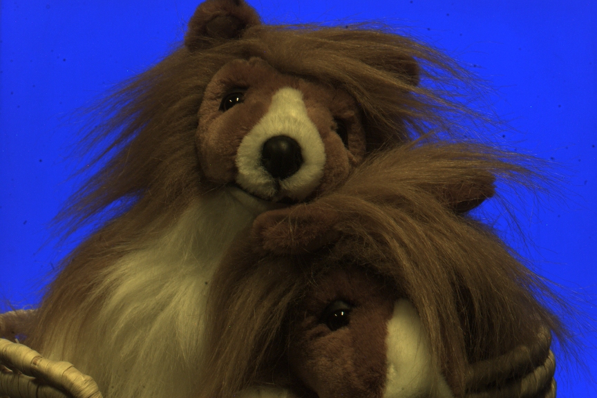
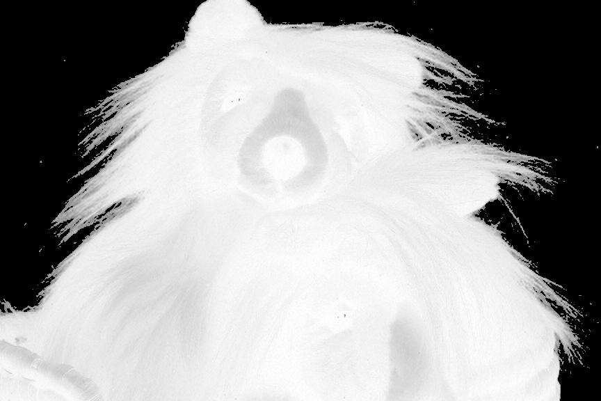
Hairs are always a good test case for matting algorithms as the ends of hairs are usually small enough to be captured by camera (resolution dependent) and prove challenging for image matting algorithms. \ The Vlahos matting technique is also more robust than the difference matte technique as the problem space has been constrained down to just blue/green pixels for the background - It also does not require a clean plate to work.

Triangulation

This is a technique developed by Smith and Blinn where they observed that the same foreground $F$ photographed in front of two different background $B_{1}$ and $B_{2}$ would yield an overdetermined system of linear equations involving two unknown ( $\alpha$ and $F$ ) as defined by the following equations

I_{1} = \alpha F + (1 - \alpha)B_{1} \\ I_{2} = \alpha F + (1 - \alpha)B_{2}

Solution to Triangulation using the System of Linear Equations

Another way to view the triangulation equations is to represent it in the matrix form $Ax=b$ where $x = [r_{F} \space g_{F} \space b_{F} \space \alpha_{F}]^{T}$ and $b = [r_{\delta 1} \space g_{\delta 1} \space b_{\delta 1} \space r_{\delta 2} \space g_{\delta 2} \space b_{\delta 2}]^{T}$ . We define $\delta$ as the difference between the image and the background i.e $r_{\delta 1} = r_{I_{1}} - r_{B_{1}}$ at that particular pixel location. \ The entire problem can then be viewed as

\left[ {\begin{array}{cccc} 1 & 0 & 0 & -r_{B_{1}} \\ 0 & 1 & 0 & -g_{B_{1}} \\ 0 & 0 & 1 & -b_{B_{1}} \\ 1 & 0 & 0 & -r_{B_{2}} \\ 0 & 1 & 0 & -g_{B_{2}} \\ 0 & 0 & 1 & -b_{B_{2}} \\ \end{array} } \right] * \left[ {\begin{array}{c} r_{F} \\ g_{F} \\ b_{F} \\ \alpha_{F} \\ \end{array}} \right] = \left[ {\begin{array}{c} r_{\delta 1} \\ g_{\delta 1} \\ b_{\delta 1} \\ r_{\delta 2} \\ g_{\delta 2} \\ b_{\delta 2} \\ \end{array}} \right] \\ Ax = b

As $A$ is not a square matrix but a $(6 \times 4)$ matrix, finding its inverse is going to be difficult. One way to circumvent this, is to find its generalised left inverse $(A^{T}A)$ which is invertible. \ Therefore, the system becomes the least squares solution

(A^{T}A)x = A^{T}b \\ x = (A^{T}A)^{-1}(A^{T}b) \\ \dot{.\hspace{.095in}.}\hspace{.5in} \left[ {\begin{array}{c} r_{F} \\ g_{F} \\ b_{F} \\ \alpha_{F} \\ \end{array}} \right] = (A^{T}A)^{-1}(A^{T}b)

This can be implemented in code as

import numpy as np
from PIL import Image 

def transform(imgs):
    imgs = map(lambda x: np.array(x), imgs)
    return [x/255.0 for x in imgs]

def triangulate(c1, c2, b1, b2):
    c1, c2, b1, b2 = transform([c1,c2,b1,b2])
    img_shape = (c1.shape[0], c2.shape[1])
    mask = np.zeros((*img_shape,3), dtype=np.float)
    alpha = np.zeros(img_shape, dtype=np.float)
    '''
    Writing the problem as 
    xA = b
    x(AA^T) = bA^T
    x = (b.A^T)(AA^T)^-1
    '''
    d1 = c1 - b1 
    d2 = c2 - b2
    for i in range(img_shape[0]):
        for j in range(img_shape[1]):
            A = np.array([
                [1, 0, 0, 1, 0, 0],
                [0, 1, 0, 0, 1, 0],
                [0, 0, 1, 0, 0, 1],
                [-b1[i,j,0], -b1[i,j,1], -b1[i,j,2], -b2[i,j,0], -b2[i,j,1], -b2[i,j,2]]
            ])

            b = np.array([
                [d1[i,j,0], d1[i,j,1], d1[i,j,2], d2[i,j,0], d2[i,j,1], d2[i,j,2] ]
            ])
            
            x_1 = np.dot(b, A.T)
            x_2 = np.linalg.inv( np.dot(A,A.T) )
            x = np.dot(x_1, x_2)
            x = np.clip(x, 0, 1)
            
            mask[i,j,:] = np.array([x[0,0], x[0,1], x[0,2]])
            alpha[i,j] = x[0,3]

    mask = np.array(mask * 255, dtype=np.uint8)
    alpha = np.array(alpha * 255, dtype=np.uint8)
    return (mask, alpha)

b1 = Image.open('flowers-backA.jpg')
b2 = Image.open('flowers-backB.jpg')
c1 = Image.open('flowers-compA.jpg')
c2 = Image.open('flowers-compB.jpg')

mask, alpha = triangulate(c1, c2, b1, b2)
mask = Image.fromarray(mask)
alpha = Image.fromarray(alpha)

mask.show()
alpha.show()

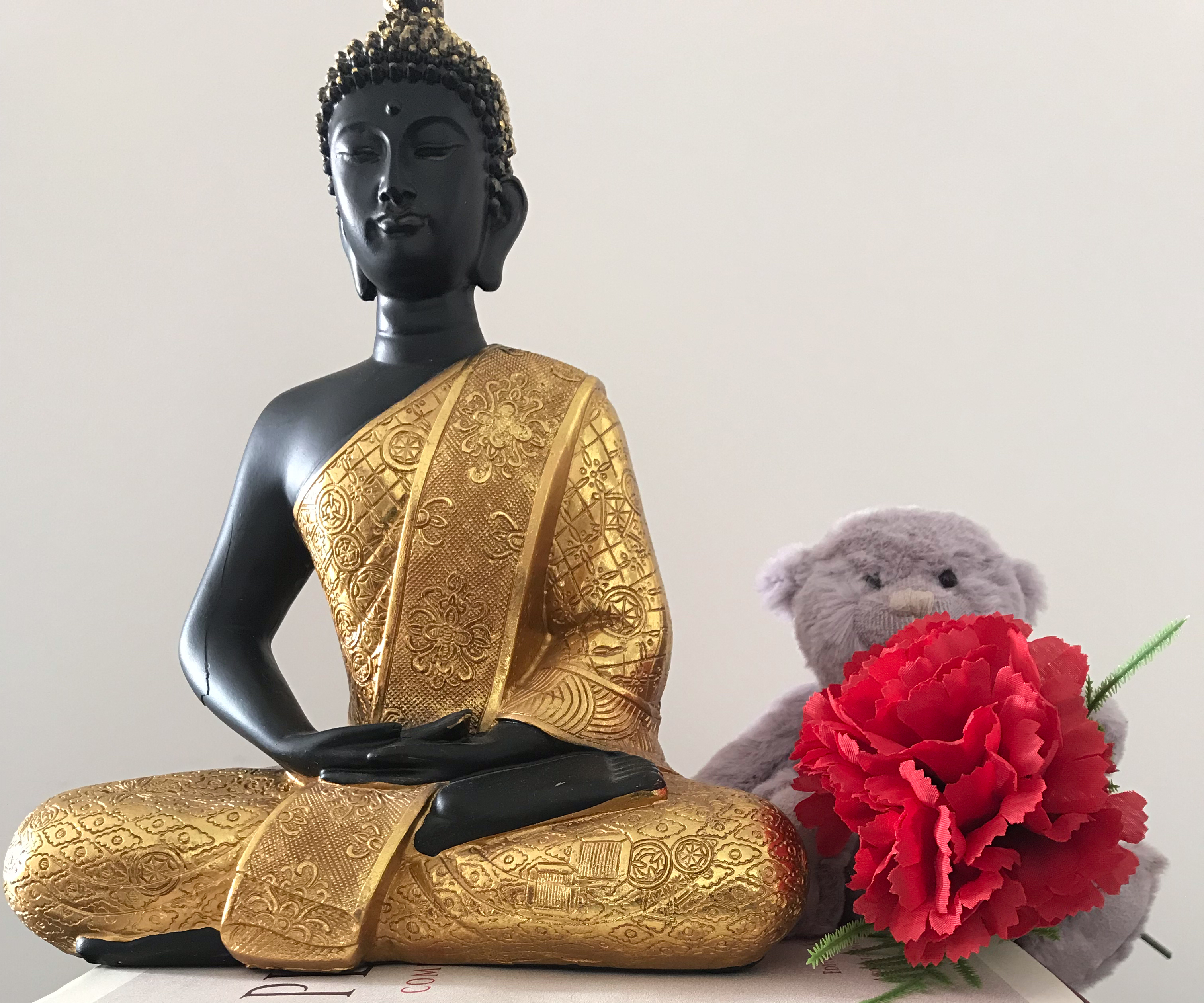
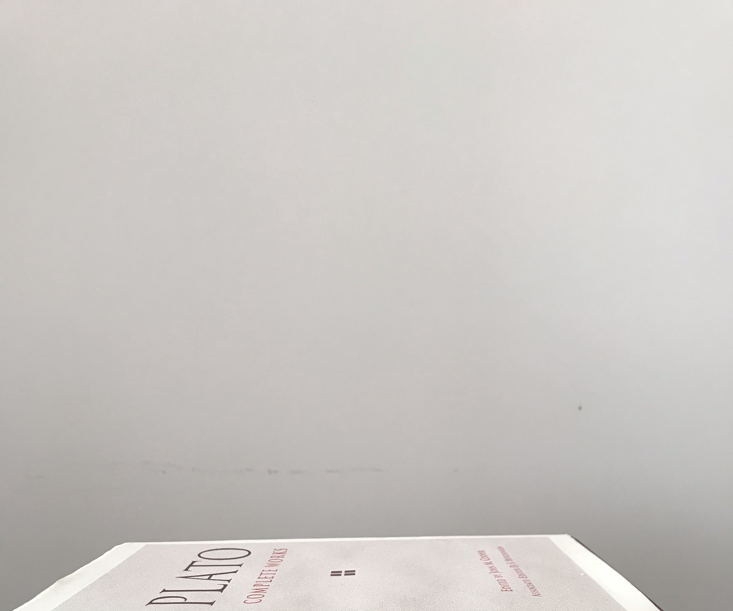
Let the backgrounds be

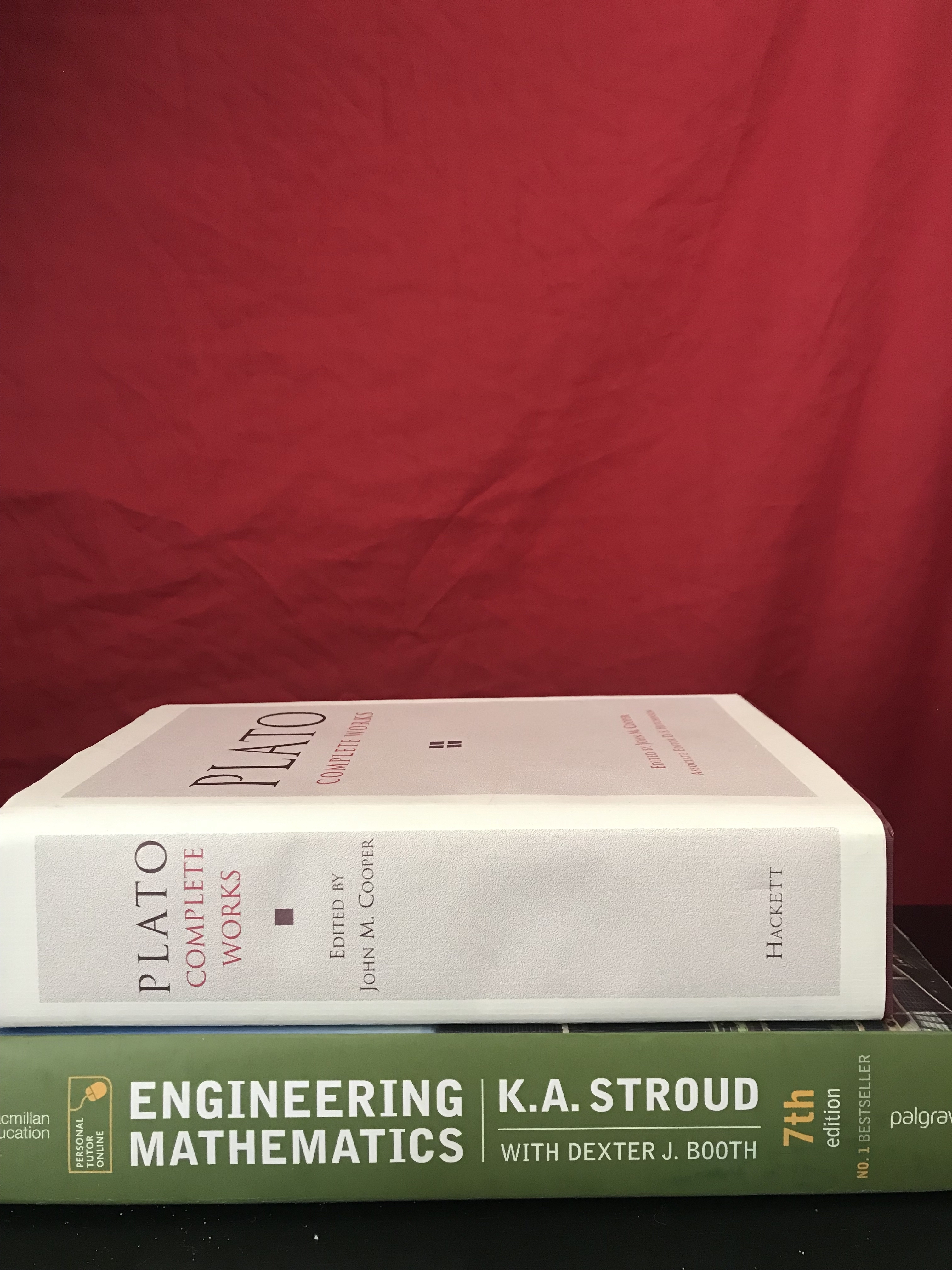
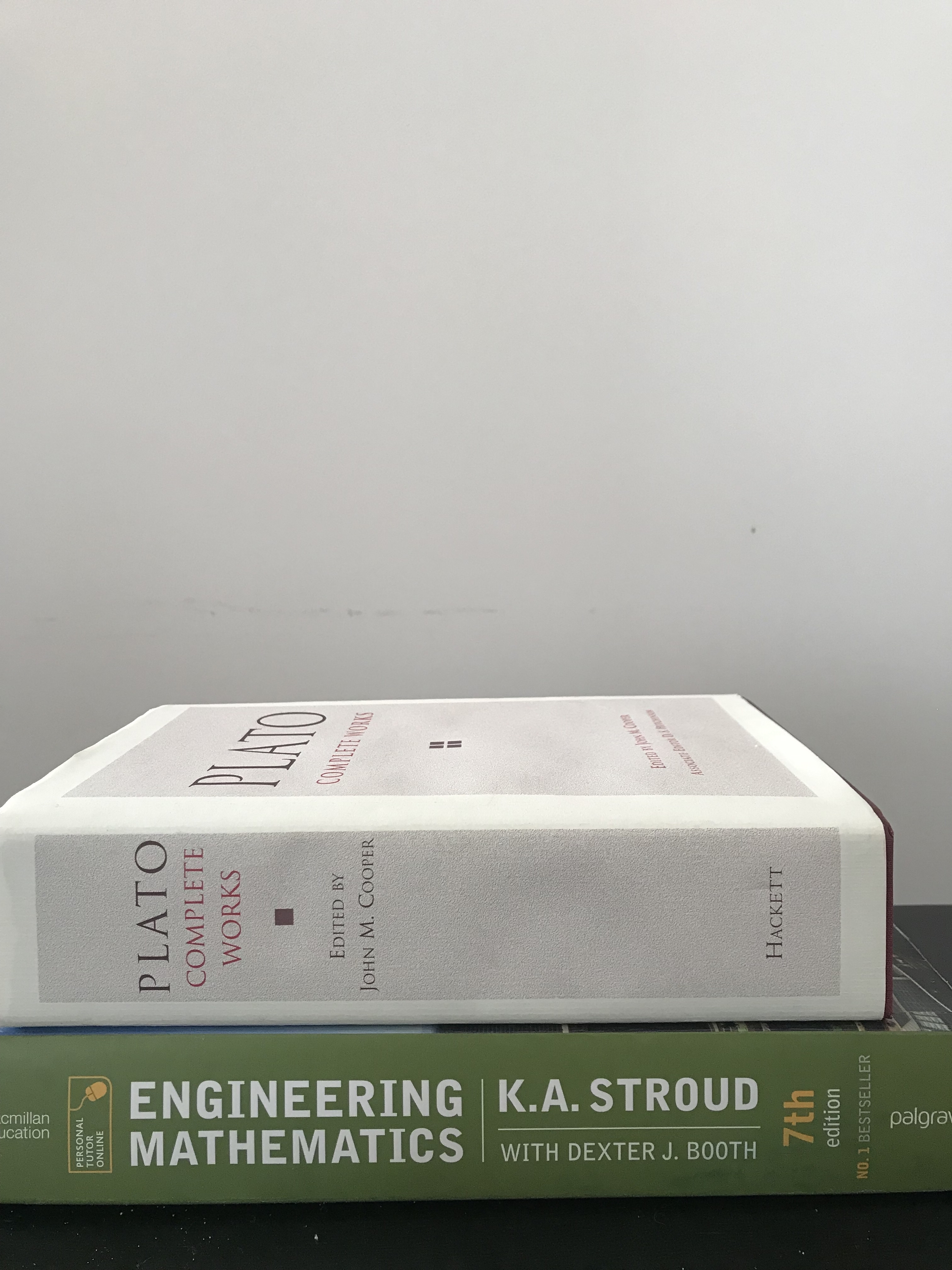
And the input images with the foreground object and the respective backgrounds be

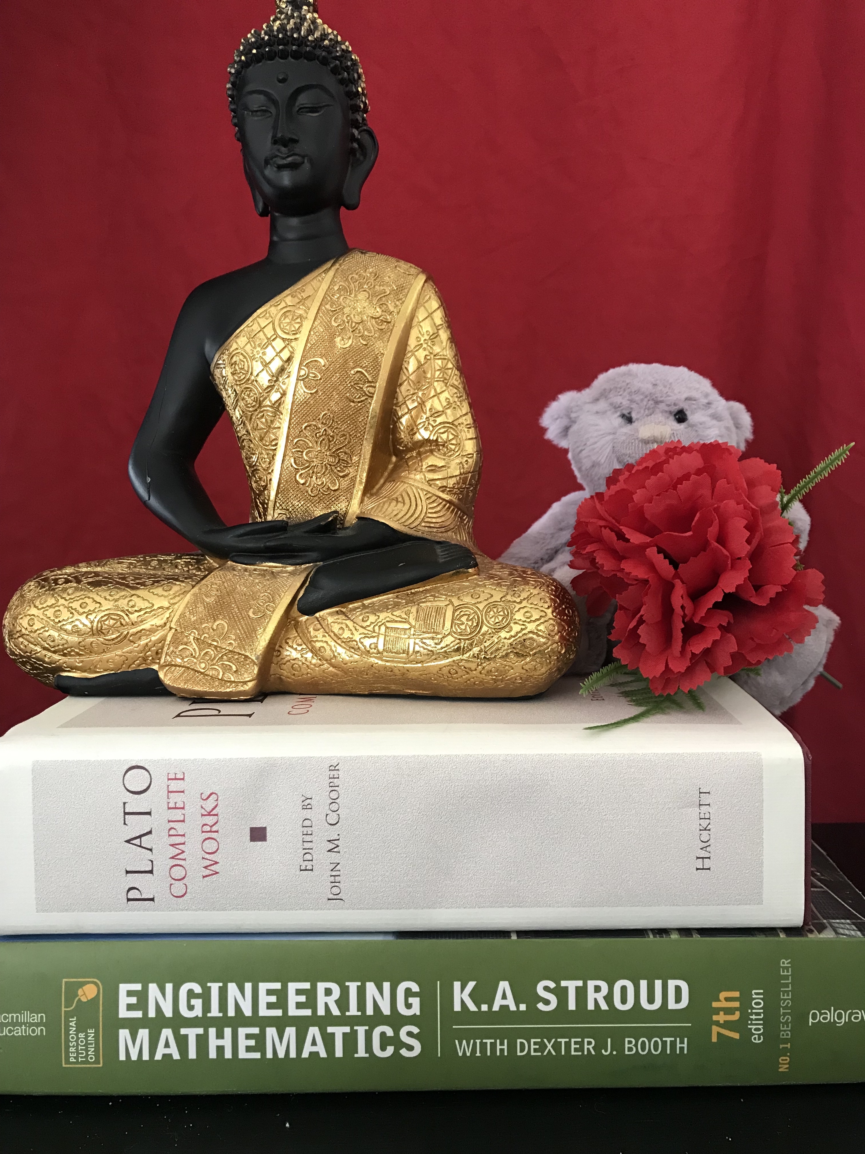
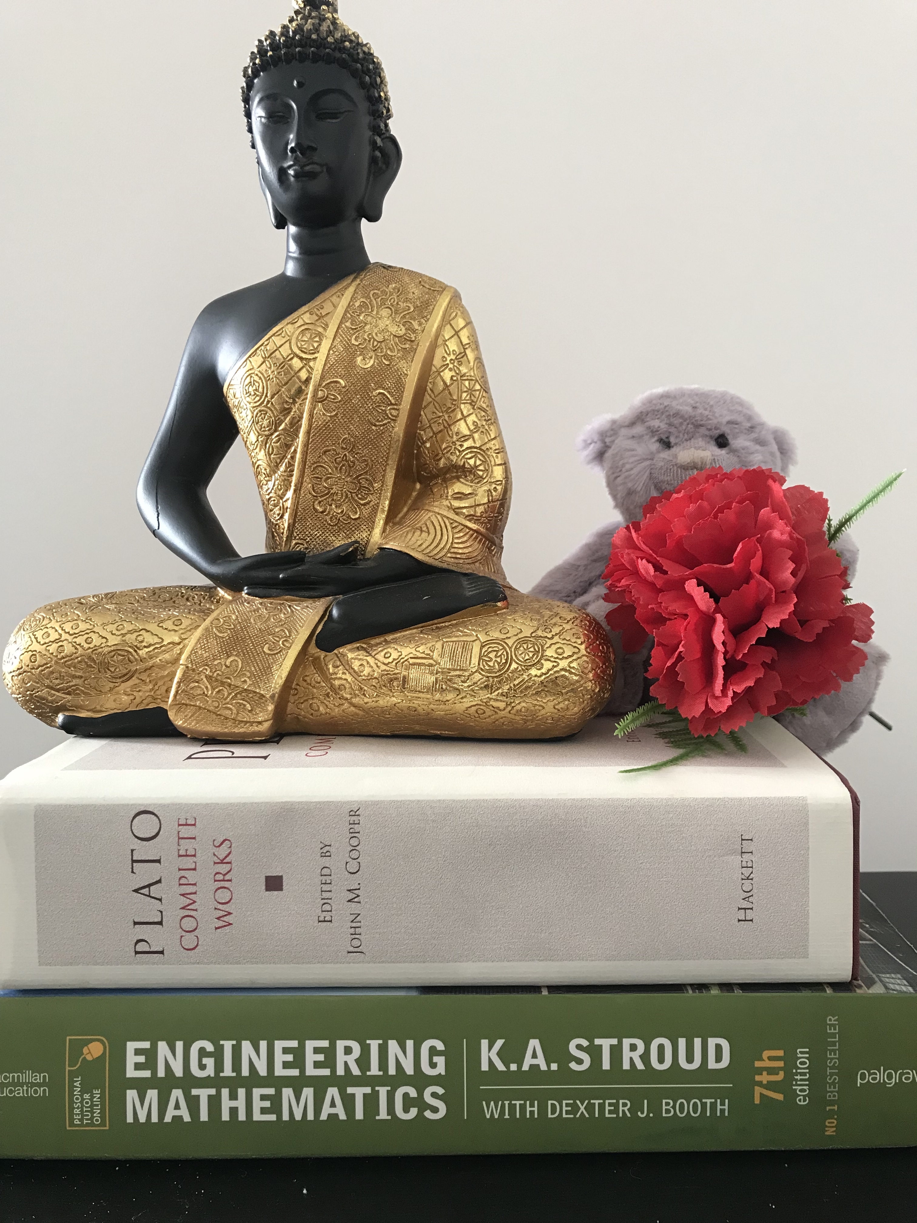
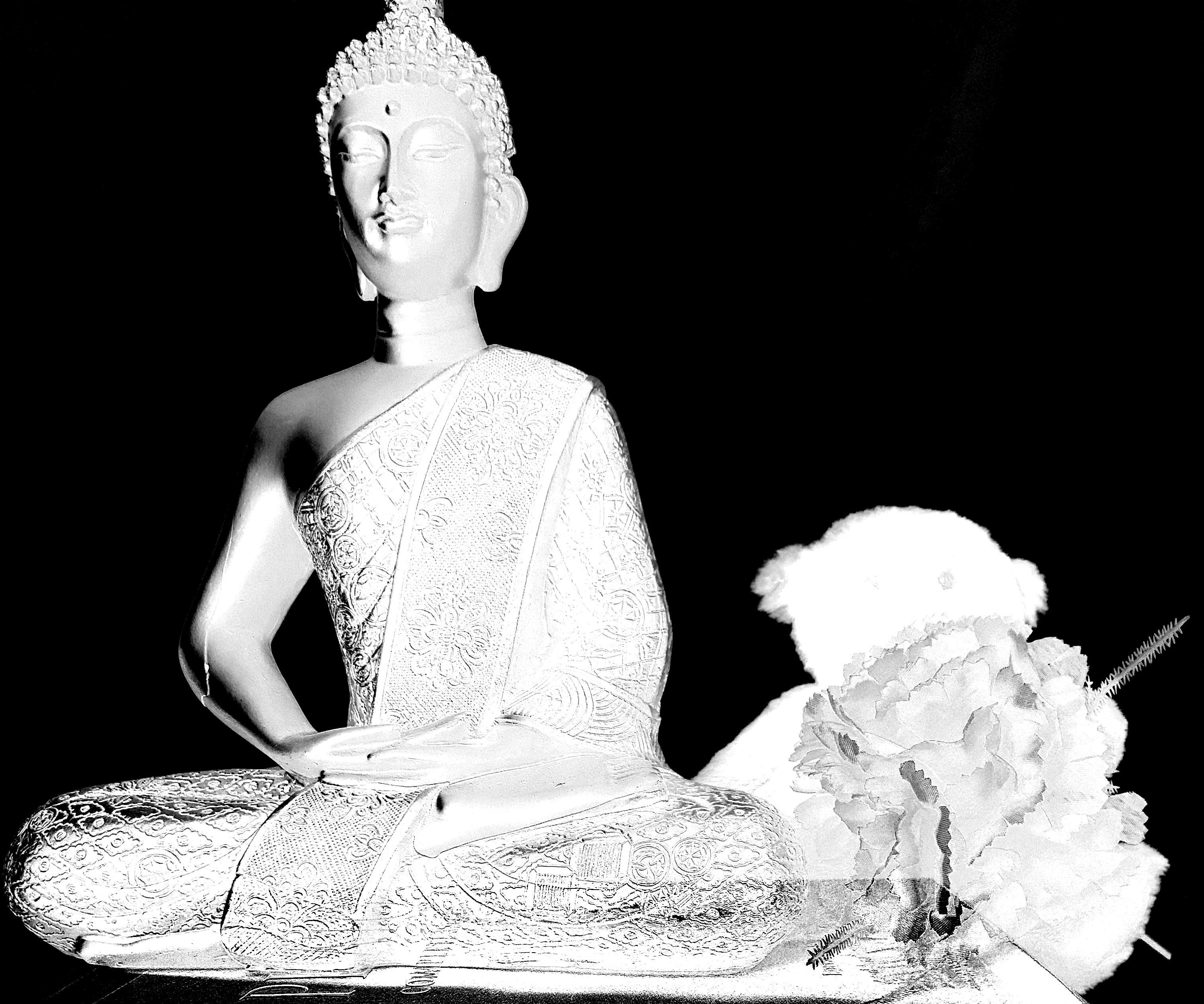
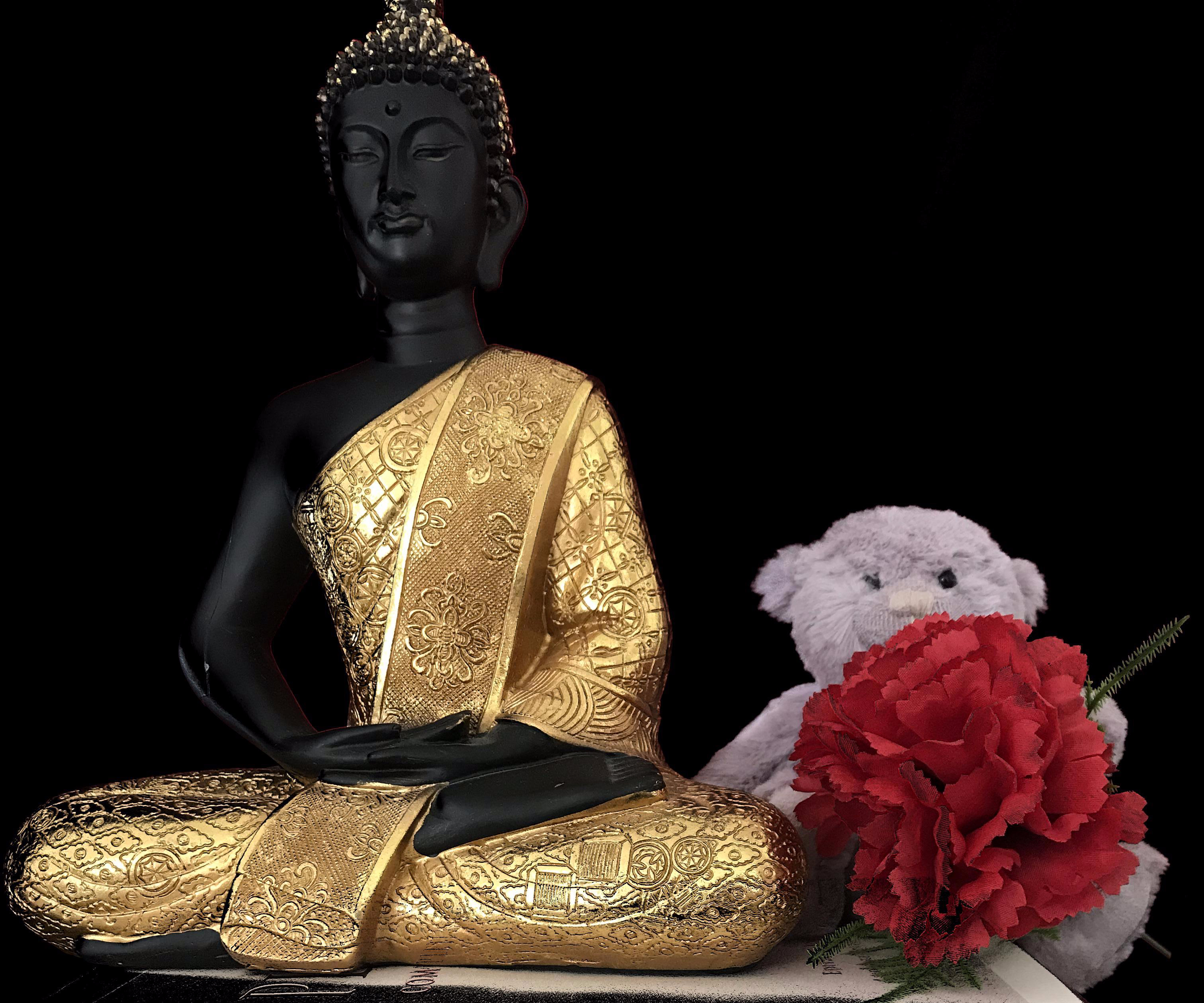
Using the code above, we can compute the alpha Matte and Foreground as

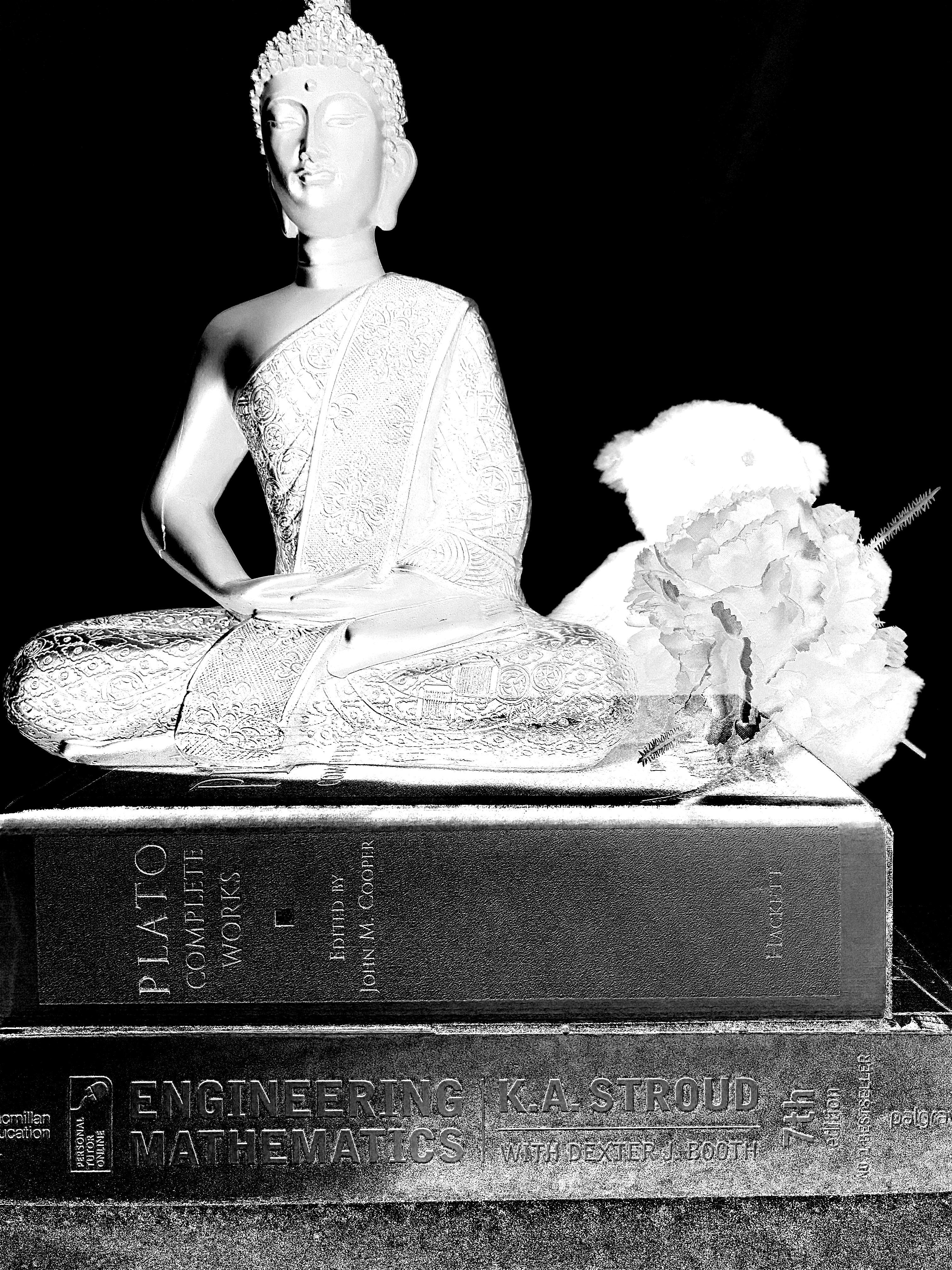
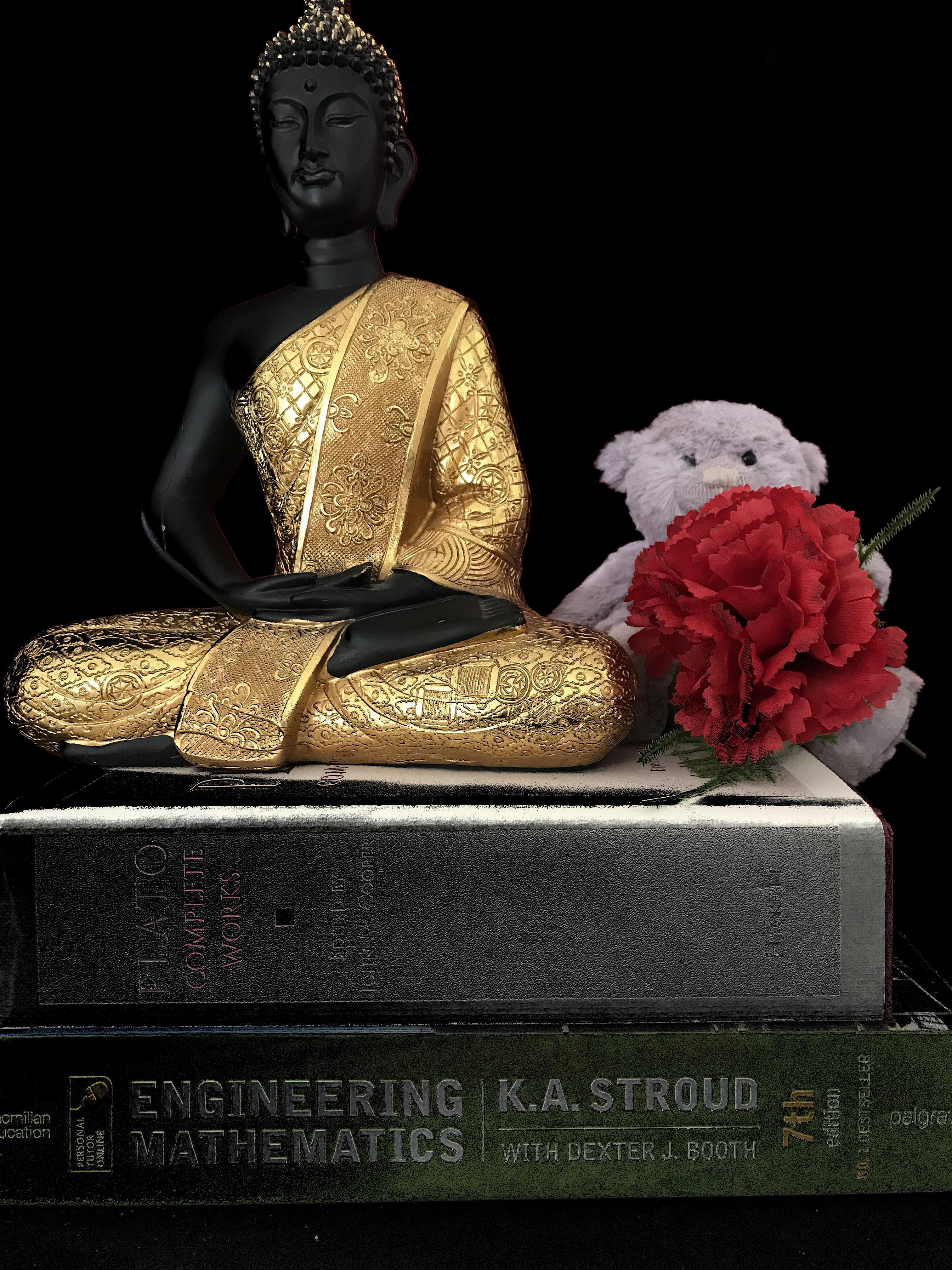
Ideally i would have cropped out the regions with the textbooks as they muddy the results but I thought it best to leave it there so the reader is informed of the possibility of errors creeping into the result. \ Some possible sources of errors are the changes in lighting and slight camera movement.

Faster Solution to Triangulation by Generalisation of the Formula

The code given above for computing the alpha and foreground using the triangulation technique can be slow depending on the image size due to the fact that the pseudo-inverse is computed at each pixel location. A faster solution can be derived using the triangulation system of equations that operates on the entire image, we can define an equation for $\alpha$ as

I_{1} = \alpha F + (1 - \alpha)B_{1} \\ \alpha F = (1 - \alpha)B_{1} - I_{1} \\

Repeating the same for the second image and using $F$ as the common term, we now have

\alpha F = (1 - \alpha)B_{2} - I_{2}

Therefore, by equating $\alpha F$ from both equations, we have

(1 - \alpha)B_{1} - I_{1} = (1 - \alpha)B_{2} - I_{2} \\ (1 - \alpha)B_{1} - (1 - \alpha)B_{2} = I_{1} - I_{2} \\ (1 - \alpha)(B_{1} - B_{2}) = (I_{1} - I_{2}) \\ 1 - \alpha = \frac{(I_{1} - I_{2})}{(B_{1} - B_{2})} \\ \alpha = 1 - \frac{(I_{1} - I_{2})}{(B_{1} - B_{2})} \\

Some derivations do rationalise the fractions to produce

\alpha = 1 - (\frac{(I_{1} - I_{2}) \times (B_{1} - B_{2})}{(B_{1} - B_{2}) \times (B_{1} - B_{2})})

And its implementation is shown as

def triangulate_faster(c1, c2, b1, b2):
    c1, c2, b1, b2 = transform([c1,c2,b1,b2])
    alpha = np.sum((c1 - c2) * (b1 - b2), axis=2) / np.sum((b1 - b2)**2, axis=2)
    alpha = 1 - alpha
    alpha = np.clip(alpha, 0, 1) 
    alpha = np.array(alpha * 255, dtype=np.uint8)

    mask = np.zeros(c1.shape, dtype=np.uint8)
    mask[:,:,0] = np.multiply(c1[:,:,0], alpha)
    mask[:,:,1] = np.multiply(c1[:,:,1], alpha)
    mask[:,:,2] = np.multiply(c1[:,:,2], alpha)

    return mask, alpha

Image Matting Resources

Alpha Matting website: Contains a dataset, sample code and an online benchmark