The You only look once (YOLO) algorithm is the first in a series of 4 iterations of the algorithm. Developed by Joseph Redmon et al, it was the first novel object detection algorithm that performed detection using a unified end-to-end neural network in period of multi-stage detectors.

This tutorial will show you how to train an object detection deep neural network using the first version of the YOLO algorithm (YOLOv1) from scratch. It would also explain how to augment your dataset, the loss function used and how to perform inference using the PyTorch framework.

Object Detection

The problem of determining what is in a given image and where, is a challenging problem in Computer Vision that has been worked on since the early 1990s. In formal terms, the task in object detection is to compute a bounding box around objects we are interested in and also determine the classes the objects belong to (e.g humans, cars, dogs etc).

Early attempts in Object detection consisted of hand crafter classifiers such as the Viola-Jones detector and gradually evolved to learning based methods such as the R-CNN. The paper, Object Detection in 20 Years: A Survey, by Zou et al provides a very good overview on the history of object detection from 1990s to 2019.

Deep Learning in Object Detection

Following the success of convolutional neural networks in the ImageNet (ILSVRC) challenge in 2012 (remember AlexNet). Girshick et al proposed RCNN which leaped forward the field of object detection after years of stagnation. RCNN and other multi stage detectors learning based detectors usually consisted of

• A region proposal function that generates potential regions (bounding boxes) e.g using selective search.
• An image is taken from each proposed region and used as inputs to a CNN model (usually pretrained on ImageNet) which then outputs a fixed set of features.
• These features are then fed into another classifier such as a Support Vector Machine (SVM) that predicts an object class given features from the CNN output.
• Some algorithms do have a last step, where another classifier e.g linear regressor is used to refine the bounding box coordinates

The 'You Only Look Once (YOLO)' algorithm

YOLO (available online at arXiv:1506.02640) unifies all the stages of the multi-stage object detectors and as a result it is a much more simpler algorithm and a lot faster to train. It uses a single deep convolutional network to directly predict the class probabilities and boinding boxes. YOLOv1 was extremely fast compared to the other deep learning detectors at the time, per the author, it runs at 45 frames per second (fps) on a Titan X GPU.

This adaptation of YOLOv1 uses some modern techniques borrowed from later versions to make this current version more robust during training. Techniques such as data augmentation, Global average pooling and Batch Normalisation were used. This current version of YOLO while being fast does struggle with localisation accuracy compared to other multi-stage detectors like RCNN, although these issues would fixed in later versions v2, v3 & v4 (recently released in 2020).

How It Works

This section explains how YOLO performs unified detection. Without a selective search algorithm to propose bounding boxes, YOLO divides the entire image into a grid and predicts bounding boxes at each grid cell. The predictions at each grid cell contains all the revelant information needed to localise and determine object classes in the image. This is explained in greater detail as a series of the following steps

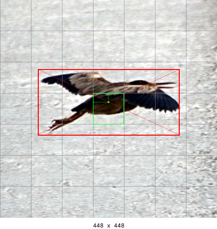
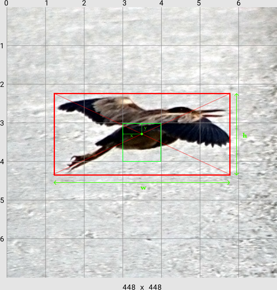
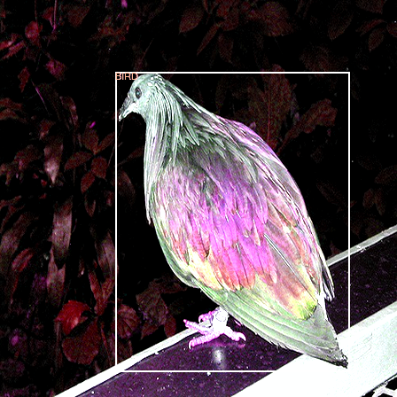
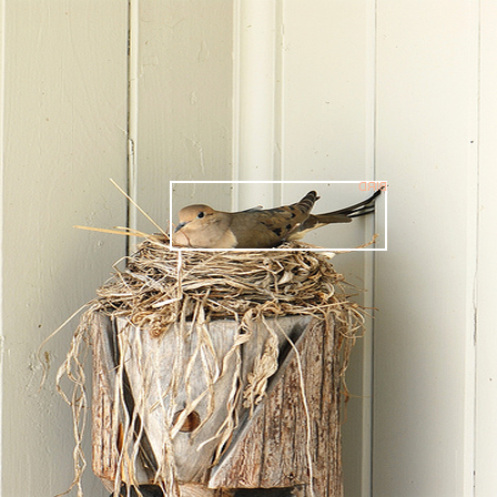
• An object center is assigned to each object in a given image. This center is chosen by dividing the input image into an $S \times S$ grid. If the center of an object in the image falls into a particular grid cell then that grid cell is responsible for detecting that object. In the $448 \times 448$ image below, the image is divided into a $7 \times 7$ grid ($S = 7$). As there is only 1 object, a bird, in this image, the grid cell responsible for predicting the bird is the $(4,4)$ grid cell. This was chosen based on the cross center of the bounding box drawn over the bird falling in that position.

• The CNN outputs a prediction tensor of the size $S \times S \times (B * 5 + C)$ where $S,S$ are the spatial dimensions, $B$ is the number of bounding box predictions you want at each cell (the bounding box with the highest confidence is chosen for the final prediction), $C$ is the number of classes in your dataset and 5 represents the bounding box coordinates along with the confidence of the classifier. 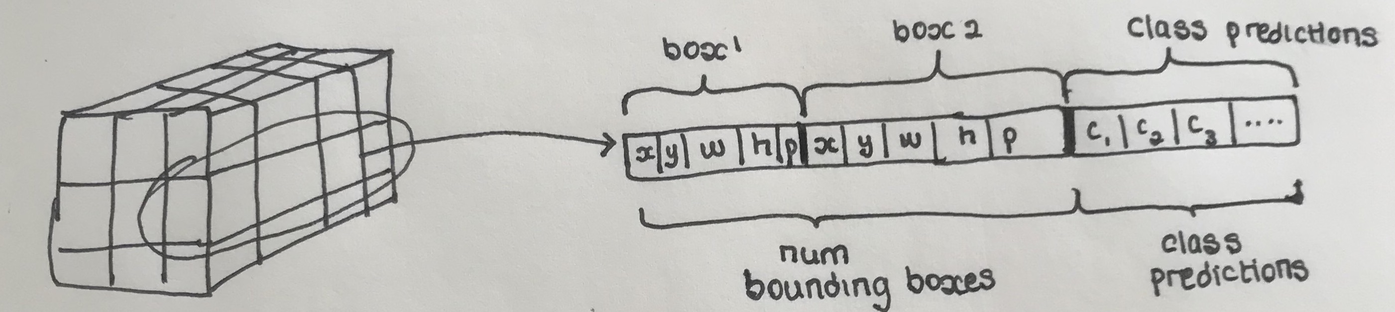The number of bounding boxes, $B$, you want at each cell can be arbitrary and more bounding boxes makes the model slightly more accurate but remember that increasing B also increases the computational and memory costs.

• Each grid cell prediction contains $B$ number of bounding boxes and $C$ class predictions

  • A bounding box prediction consists of 5 elements: The $x,y,w,h$ values of the bounding box and $p$, the probability that there is an object whose center falls within this grid cell (this is different from what is in $C$, which is the probability that the object belongs to a certain class). 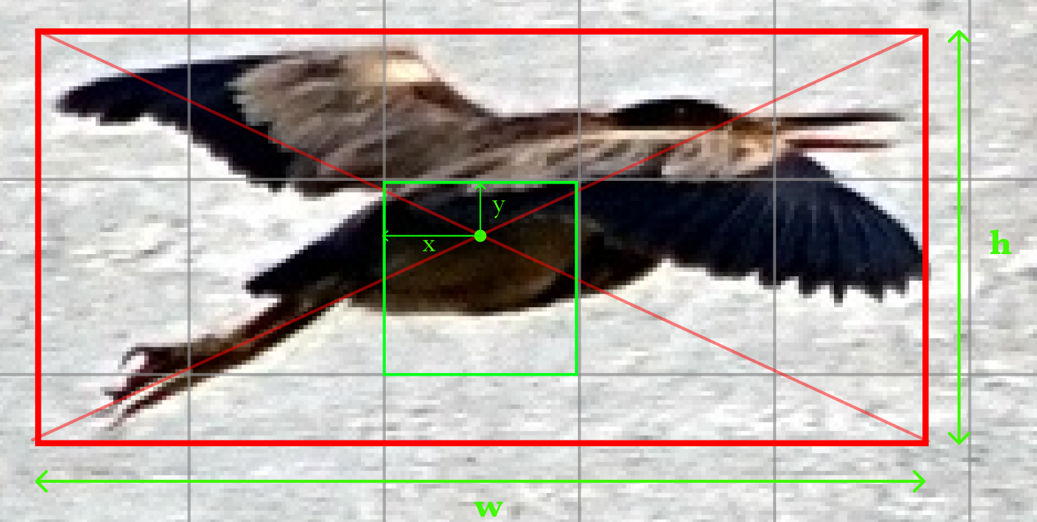The $x,y$ coordinates of the bounding box are predicted relative to the grid cell and not the entire image but the width and height ($w,h$) are predicted relative to the entire image.

    Increasing the number of bounding boxes also increases the number of computations for prediction and training.

  • Each grid cell also predicts the probability of the detected object belonging to a specific class $class_i$ given that it is confident there is an object whose's center is in the grid cell and this information is all contained in $C$.

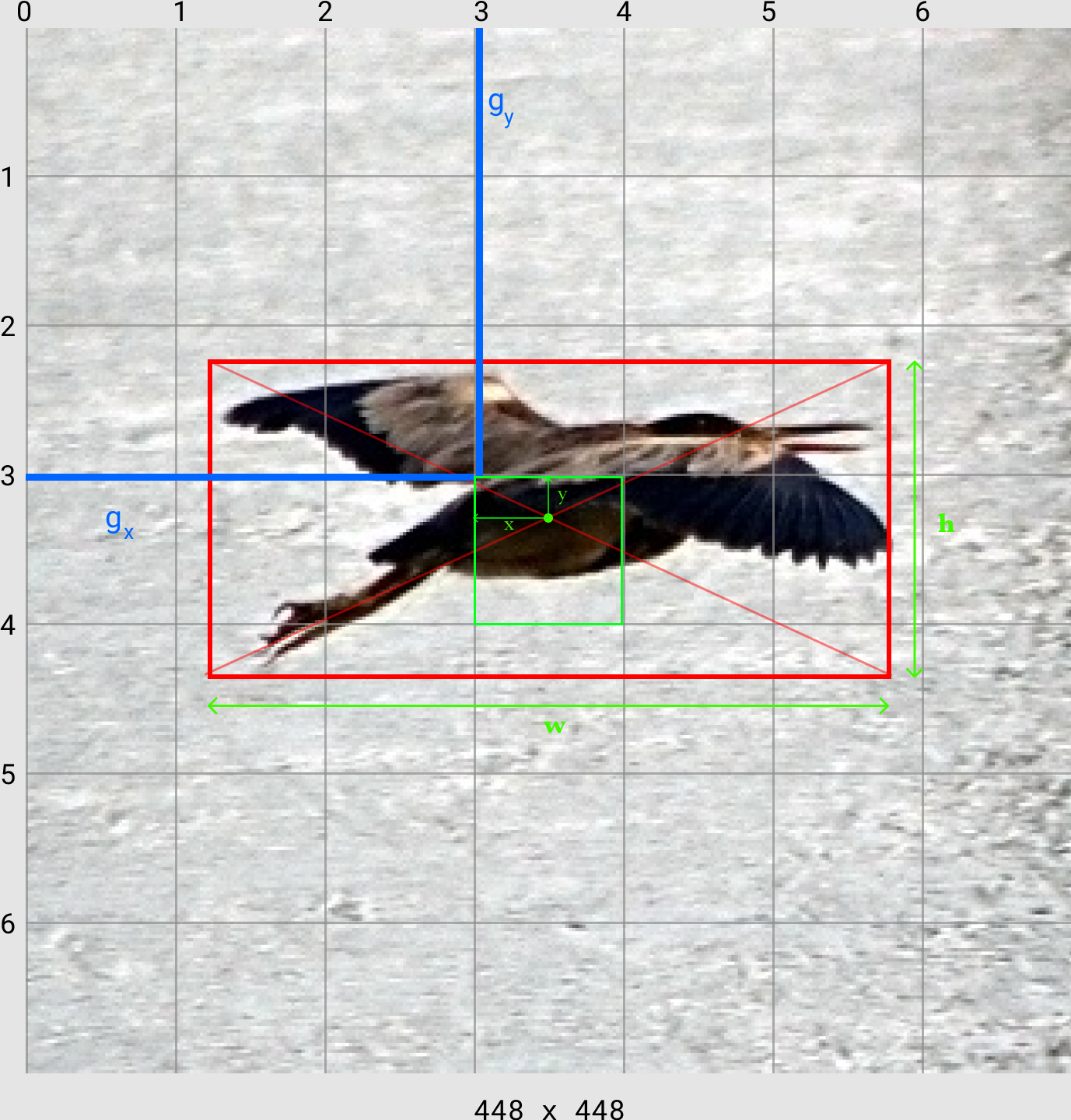
• For use later in loss calculations, the ground truth bounding box cordinates are all parameterised to be between 0 and 1. The width and height of the bounding box are calculated as a ratio of the entire image's width and height. The ($x,y$) grid cell offsets are parameterised as a ratio of a grid's width and height. For example, given the a $448 \times 448$ image and $S = 7$. By dividing the width/height by the grid size, we have a grid dimension where each grid cell is $64 \times 64$ pixels wide. Therefore a bounding box from our dataset with $x = 32, y = 16, width = 300$ and $height = 150$, would be parameterised as

  $$x = \frac{32}{64}, y = \frac{16}{64}, width = \frac{300}{400} \text{ and } height = \frac{150}{448} \\$$

Using the PascalVOC dataset for object detection

The PascalVOC dataset, is a dataset for object detection, classification and segmentation. The total size on disk is about 5.17GB for the 2007 and 2012 dataset, which makes it perfect for grokking the performance of the YOLOv1 algorithm.

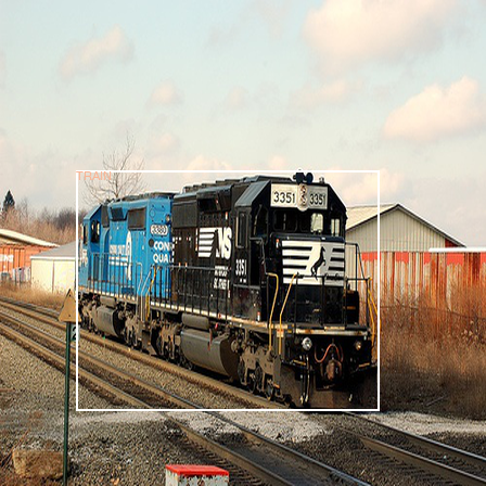
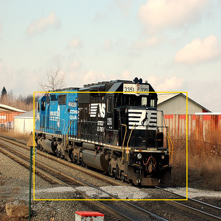
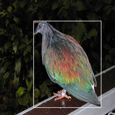
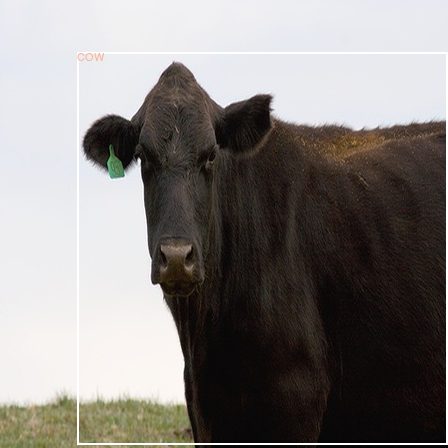
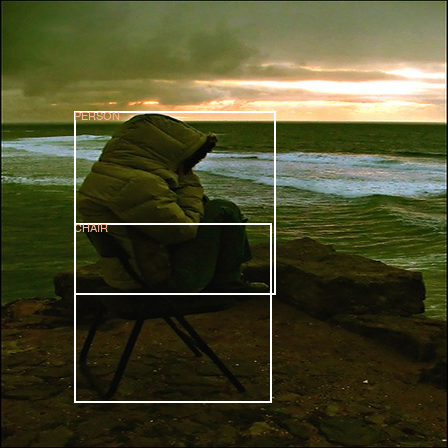
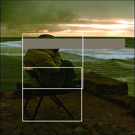
A sample image with its corresponding annotation file is shown below, the parts of the annotation file to observe have been highlighted in red.

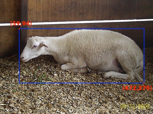
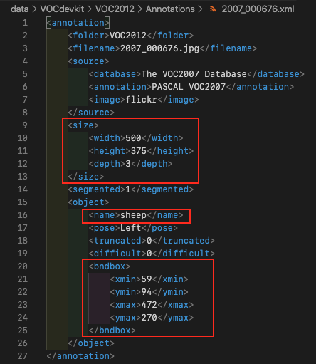
The object class is denoted in 'annotation -> object -> name' tag, and this would be one of the 20 classes in the Pascal VOC dataset ("aeroplane", "bicycle", "bird", "boat", "bottle", "bus", "car", "cat", "chair", "cow", "diningtable", "dog", "horse", "motorbike", "person", "pottedplant", "sheep", "sofa", "train", "tvmonitor"). \ The bounding boxes are encoded in the top-left and bottom-right coordinates (min-max encoding), however, based on the YOLO algorithm, predictions are made with reference to the object centers (center encoding) and not their min-max coordinates. Therefore, we need to convert from the min-max encoding in the annotation file to the bounding box center encoding for use in the YOLO algorithm.

Converting from Bounding box min-max encoding to Bounding box center encoding

To make consequent calculations easier, we normalise the bounding box coordinates to values between 0 and 1 i.e $b \in [0,1]^{4 \times 1}$. Let the bounding box coordinates in min-max encoding be defined as $b_{min-max}$ and the bounding box coordinates in center encoding be defined as $b_{center}$.

Where $W,H$ are the width and height of the image respectively, Converting from $b_{min-max}$ to $b_{center}$ can simply be defined as

This is easily implemented as

def convert(size, box):
    W = 1/size[0]
    H = 1/size[1]
    x_min, x_max, y_min, y_max = box

    x = (x_min + x_max)/2.0 * W
    y = (y_min + y_max)/2.0 * H
    w = (x_max - x_min) * W
    h = (y_max - y_min) * H

    return (x,y,w,h)

Converting from center bounding box encoding to YOLO bounding box encoding

We currently have $b_{center}$ which contains the x,y location of the object center and the width and height of the object, scaled between 0 and 1.

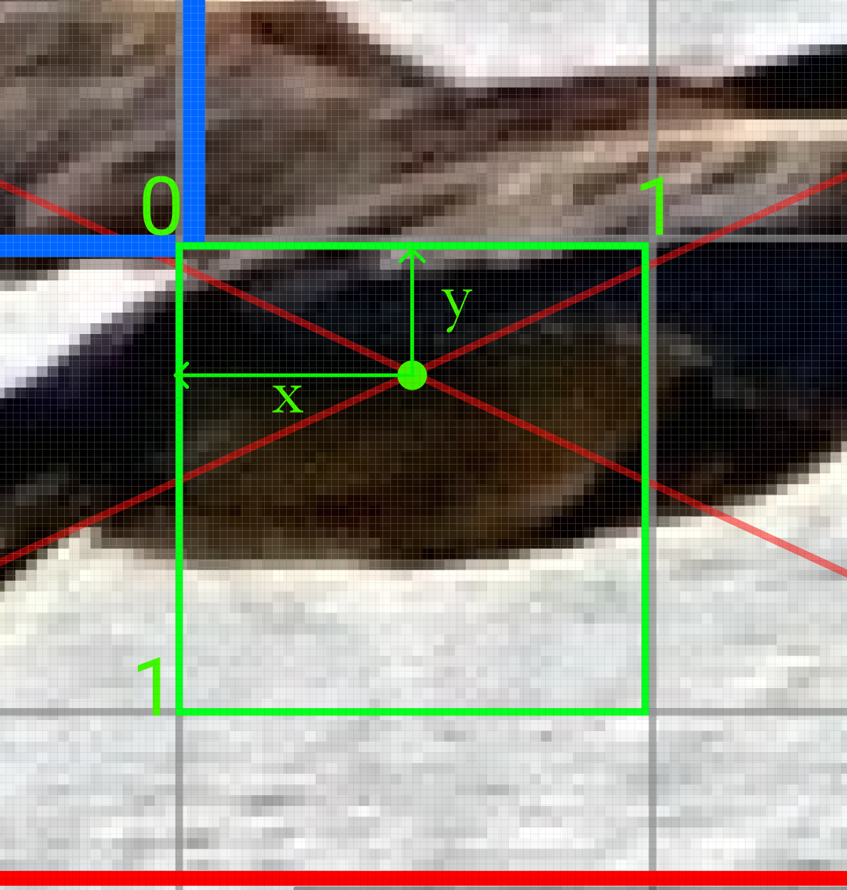
To convert this to YOLO bounding box encoding ($b_{yolo}$) which takes the x,y location of the object center (relative to the image's width and height) and converts it to an (x,y) coordinate relative to the grid cell (fig 3). The width and height are left as they are in the YOLO encoding.

This is formalised as

During the loss calculations, the square root of the width, $\sqrt{w}$ and height, $\sqrt{h}$ are used as they ensure stability and prevent the loss function from penalising small width and height predictions.

In our implementation, we assume that the model outputs bounding box coordinates in $b_{yolo}$, therefore we convert to $b_{center}$ for loss calculations as that was much easier to do. Therefore, each observation from the dataset is encoded as

def batch_collate_fn(batch):    
    images = [item[0].unsqueeze(0) for item in batch]    
    
    detections = []
    for item in batch:
        det = item[1]
        image_detections = torch.zeros(1, _GRID_SIZE_, _GRID_SIZE_, 5)
        for cell in det:            
            gx = math.floor(_GRID_SIZE_ * cell[1])
            gy = math.floor(_GRID_SIZE_ * cell[2])
            
            image_detections[0,gx,gy,0:4] = cell[1:]
            image_detections[0,gx,gy,4] = cell[0]
        detections.append(image_detections)

    images = torch.cat(images,0)
    detections = torch.cat(detections,0)    
    return (images, detections)

Data Augmentation

Data augmentation introduces variation into our training dataset without increasing the number of observations. This can help introduce invariance into the network and also increase its accuracy. \ The most recent version of YOLO (v4), attributes part of its increase in average precision (AP) to the modern data augmentation techniques it used, which they termed the Bag of Freebies (BoF), a repository of pixel-wise adjustments e.g CutMix, CutOut.

The following Data augmentation were used in our implementation

Color Jitter

This augmentation changes the brightness, contrast and saturation of the image, a detailed documentation on this augmentation is available on the PyTorch torchvision documentation page

As we do not depend a lot on the color information in our training example, it is fine to shift the colors around so that the network does not overfit on the color information. The parameters used in our implementation is shown below.

transforms.ColorJitter(brightness=0.5, contrast=0.5, saturation=0.5, hue=0.25)

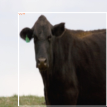
Random Blur

Here a Gaussian blur is applied to the image to reduce the amount of detail in the image so the network learns higher level information about the objects such as their shapes and distinguishing features. The documentation for the gaussian function used is available at the PIL ImageFilter documentation

class RandomBlur(object):
    def __init__(self, probability=0.5):
        self.p = probability

    def __call__(self, image):
        if random.random() < self.p:
            return image.filter(ImageFilter.GaussianBlur(radius=2))
        return image

Random Horizontal & Vertical Flip

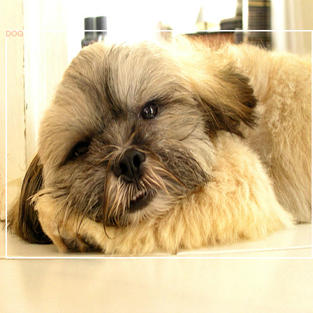
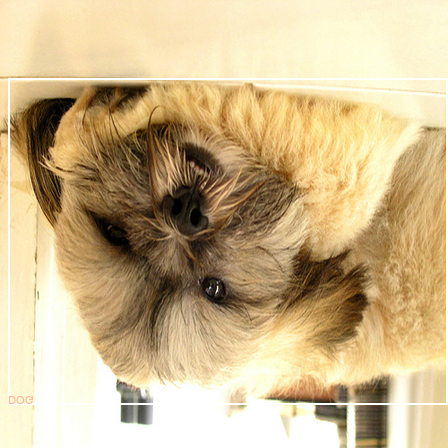
This augmentation aims to reduce dependency on the orientation of the object, as the image of a dog still contains a dog regardless of how it is positioned but sometimes it is possible the network associates a certain orientation with objects.

The image and its detection annotations are both modified to produce the horizontal and vertical flip. PyTorch's vertical flip function and PIL's transpose function were both used.

class RandomHorizontalFlip(object):
    def __init__(self, probability=0.5):
        self.p = probability

    def __call__(self, items):
        if random.random() < self.p:
            img, det = items
            img = img.transpose(PIL.Image.FLIP_LEFT_RIGHT)
            for idx,bbox in enumerate(det):
                det[idx,1] = 1 - bbox[1]
            return (img, det)
        else:
            return items


class RandomVerticalFlip(object):
    def __init__(self, probability=0.5):
        self.p = probability
        self.t = transforms.RandomVerticalFlip(p=1)

    def __call__(self, items):
        if random.random() < self.p:
            img, det = items
            img = self.t(img)
            for idx,bbox in enumerate(det):
                det[idx,2] = 1 - bbox[2]
            return (img, det)
        else:
            return items

Random Erasing

This technique is also referred to as CutOut. It is one of the newer data augmentation techniques also used in YOLOv4 and it's PyTorch documentation is available here. Here random rectangular regions in the image are erased, introducing a form of occlusion, further making the network more robust.

The parameters used in our implementation is shown below

erase_transform = transforms.RandomErasing(p=0.2, scale=(0.02, 0.33), ratio=(0.1, 0.1))

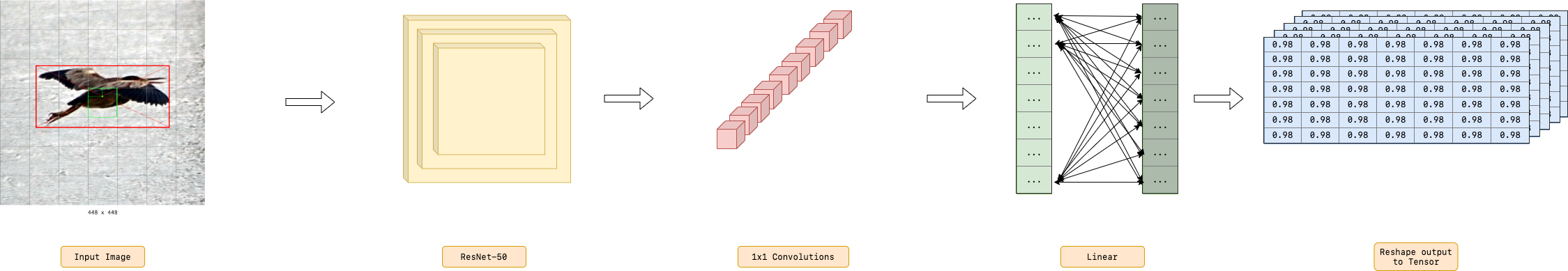
YOLO Neural Network Architecure

A pretrained ResNet50 model was used as the backbone for this YOLO architecture, this saves us the cost of training a backbone model from scratch. One thing to note regarding the backbone model is that the accuracy of the model during classification does not mean that the detector would have a higher accuracy. What matters most is the architecture of the model as a good architecture is key to having a more accurate classifier and detector.

There are some "significant" changes between the original YOLOv1 paper and ours. As my main goal is to simply the YOLOv1 algorithm and save time training, my architecture is different from the original implementation's 'backbone' and 'neck' parts of the network.

Dividing the entire network into 3 parts: The backbone which is responsible for generating features, the neck which is responsible for refining and crafting higher level semantic information and lastly the head which is responsible for making the final predictions. My network architecture is further explained in terms of these 3 parts.

• Backbone: The original paper used an architecture they developed called Darknet19 as the feature extraction network while a ResNet-50 was used in ours. This architecture is easily available in the PyTorch pretrained model repository. The paper does mention that they trained a faster version of YOLO called Fast YOLO, the premise behind making the entire CNN faster is using a faster or smaller extraction network. These extraction networks would usually have been pretrained on ImageNet as it is more computationally expensive and unstable to train from scratch in the context of object detection. A pretrained AlexNet or SqueezeNet are good candidates for a faster extraction network.
• Neck: This part of our implementation does differ significantly from the original implementation. Here we used only 2 convolutional layers and each with a batch-normalisation (BatchNorm) layer. The BatchNorm is more of a modern technique and was added to stabilise the model during training. A global average pooling was also used to ensure a fixed output size of $7\times7\times1024$ from the neck irrespective of the input image size, this is also another modern technique.
• Head: The last part is a series of linear layers (fully connected layer). Here we used 3 linear layers while the original implementation does use 2 linear layers. BatchNorm and Dropout were also used here but in hindsight having only a BatchNorm layer is better. This layer does the bounding box regression and outputs a vector of $1 \times N$ where $N$, is the product of $S * S * (B * 5 + C)$. This vector is then reshaped into a tensor of size $S \times S \times (B * 5 + C)$ to represent the predictions at each grid cell.

Defining the Model in PyTorch

Create a new file named 'YOLOv1.py' and add the following imports

import torch 
import torch.nn as nn
import torch.nn.functional as F 
import numpy as np
import ctypes
import os
from torchvision import models
from PIL import Image
from pprint import pprint

Next is to define the layers in the YOLOv1 network architecture

class YOLOv1(nn.Module):
    def __init__(self, class_names, grid_size, img_size=(448,448)):
        super(Yolo_V1,self).__init__()
        self.num_bbox = 2
        self.input_size = img_size
        self.class_names = class_names
        self.num_classes = len(class_names.keys())        
        self.grid = grid_size

        resnet50 = models.resnet50(pretrained=True)
        self.extraction_layers = nn.Sequential(*list(resnet50.children())[:-2])

        # the neck
        self.final_conv = nn.Sequential(
            nn.Conv2d(fc_in, 1024, 3, bias=False),
            nn.BatchNorm2d(1024),
            nn.Dropout2d(p=0.5),
            nn.LeakyReLU(0.1),

            nn.Conv2d(1024, 1024, 1, bias=False),
            nn.BatchNorm2d(1024),
            nn.LeakyReLU(0.1),

            nn.AdaptiveAvgPool2d((7,7))
        )
        
        # the head
        self.linear_layers = nn.Sequential(
            nn.Linear(50176, 12544, bias=False),
            nn.BatchNorm1d(12544),
            nn.Dropout(p=0.1), 
            nn.LeakyReLU(0.1),

            nn.Linear(12544, 3136, bias=False),
            nn.BatchNorm1d(3136),
            nn.LeakyReLU(0.1),

            nn.Linear(3136, self.output_size, bias=False),
            nn.BatchNorm1d(self.output_size),
            nn.Sigmoid()
        )
        

Now we can define the forward pass of the network

    def forward(self, x):

        actv = self.extraction_layers(x)
        actv = self.final_conv(actv)

        lin_inp = torch.flatten(actv)
        lin_inp = lin_inp.view(x.size()[0],-1) #resize it so that it is flattened by batch        
        lin_out = self.linear_layers(lin_inp)
        det_tensor = lin_out.view(-1,self.grid,self.grid,((self.num_bbox * 5) + self.num_classes))

        return det_tensor

Training the YOLO Neural Network

This section covers how I trained the YOLOv1 network, the missing pieces of the puzzle yet to be covered are how to choose the "best" bounding boxes amongst the ones predicted at each grid cell and the loss function used for training the network.

I trained the model on the Pascal VOC 2007+2012 dataset. Here I've set the $S \times S$, spatial values to 7, which gives us a $7 \times 7$ grid. There are 20 classes in the VOC dataset and $C = 20$. Per the YOLO paper, we also set the number of bounding boxes per grid cell, $B$, to 2. Which means the predicted tensor from the CNN would be $7 \times 7 \times 30$.

Bounding Box Selection Strategy

The output prediction tensor from the YOLO model is of size $S * S * (B * 5 + C)$. In this section, we still assume $S=7,B=2$ and $C=20$. For any arbitrary grid cell, there is a prediction of size $ 1 \times 1 \times 30$ illustrated below.

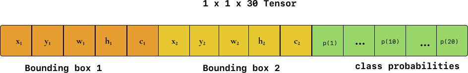
How do we decide which bounding box to use for the loss calculations at a particular cell? Let the two bounding boxes be represented as $\hat{b_1}$ and $\hat{b_2}$ and let the ground truth bounding box at that grid cell be $b$. The bounding box chosen is simply the one that has the maximum intersection over union with the ground truth. i.e

In the case where there is no ground truth prediction at that cell, we simply choose the bounding box with the highest object confidence i.e

The authors claims that this leads to specialisation between the predicted bounding boxes at a particular grid cell as one of the grid cell's bounding box predictions could specialise in predicting certain size of objects, aspect ratios or classes of object.

The box with the highest object confidence is also used to make predictions at inference time. My bounding box selection strategy is implemented in the file 'loss.py' in the corresponding Github repository for this article.

[Pro tip] When an object's center is not present at a particular grid cell, the bounding box chosen is the one with the highest confidence amongst all the bounding boxes predicted at that grid cell. This chosen bounding box is then penalised if its object confidence is not equalt to 0.

Intersection over Union (IoU)

This is also known as the Jacquard Index and it is simply a measure of how similar the predicted bounding box is to the ground truth bounding box.

This function is very important and it plays a HUGE role in our accurate our model is. In the context of the YOLO algorithm, it is what we use to select the best predicted bounding for use in loss calculations. Andrew Ng has a really good explanation of the IoU function in his video course series C4W3L06 Intersection Over Union which I highly recommend watching.

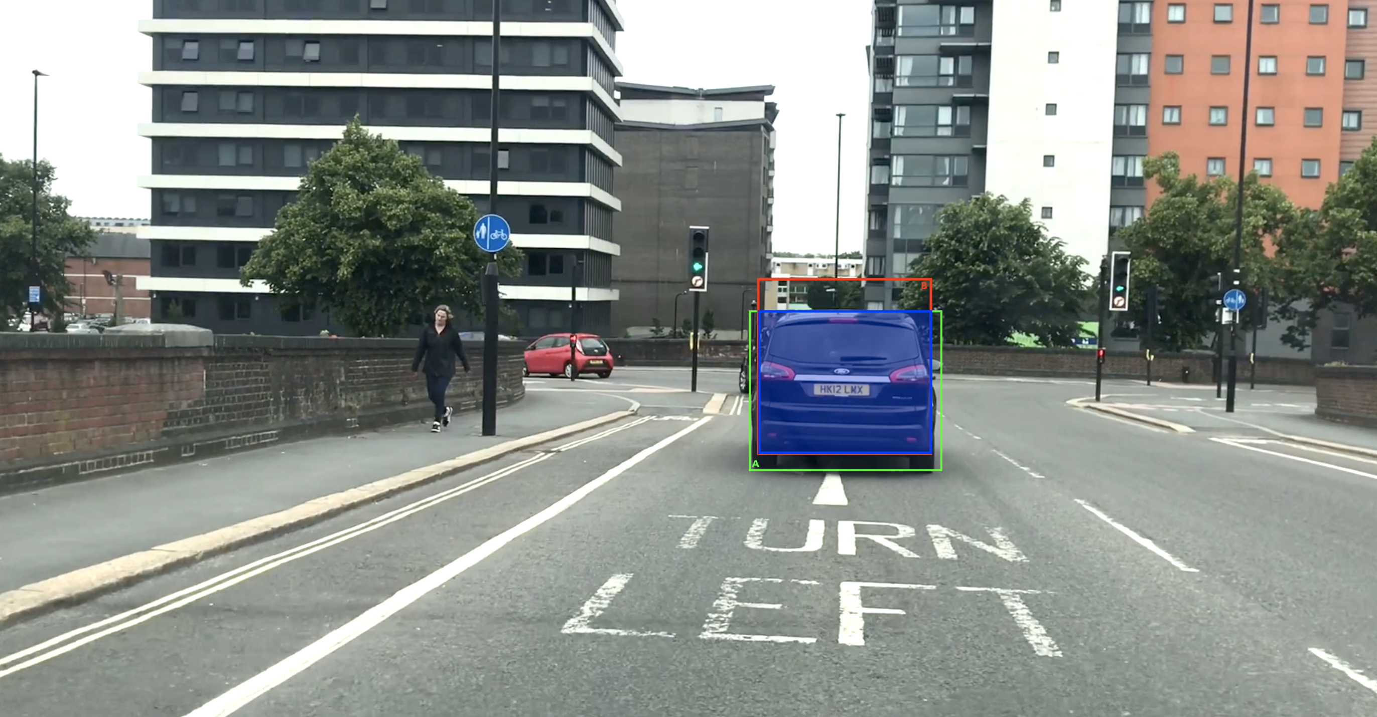
Using the diagram above, the IoU is simply the blue region as this is the area common to the green bounding box, A (ground truth) and the red bounding box, B (prediction). To give this a formal definition, it is the ratio of the area common to both boxes (blue region) to the total area of both bounding boxes.

Let the green and red bounding boxes be A, B respectively. Then their top-left and bottom right coordinates are defined as

In my implementation, the IoU function is defined as

def iou(a,b):    
    a_x_min, a_y_min = a[:,0], a[:,1]
    a_x_max, a_y_max = (a[:,2] + a_x_min), (a[:,3] + a_y_min)
    b_x_min, b_y_min = b[:,0], b[:,1]
    b_x_max, b_y_max = (b[:,2] + b_x_min), (b[:,3] + b_y_min)
    area_a = a[:,2] * a[:,3]
    area_b = b[:,2] * b[:,3]
    zero = torch.zeros(a_x_min.size()).float().to(_DEVICE_)    

My implementation is vectorised and calculates the IoU for $N$ number of bounding boxes in A and B illustrated below as

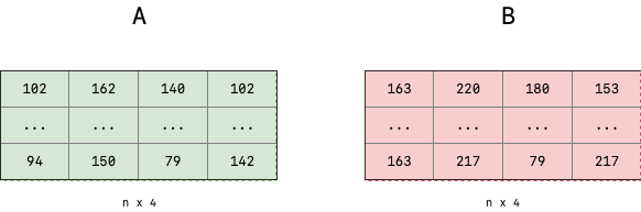
As mentioned previously, the IoU is the ratio of the common area to the total area of the bounding boxes. The width and height of the common area is defined as

inter_width = torch.max(zero, torch.min(a_x_max, b_x_max) - torch.max(a_x_min,b_x_min))
inter_height = torch.max(zero, torch.min(a_y_max, b_y_max) - torch.max(a_y_min,b_y_min))

And the intersectional area is simply the product of its intersectional width and height

inter_area = inter_width * inter_height

The total area covered by both bounding boxes A and B can be defined as

union_area = (area_a + area_b) - inter_area

Finally, the intersection over union, IoU, of A, B can be calculated as

    jac_index = inter_area / union_area    
return jac_index

One thing to note is that recent papers how shown how flawed this "bare" IoU definition is in the context of object detection See the following papers

• IoU loss: Here the IoU is used as the loss function as opposed to the one defined in the next section which is regression loss as it treat the x,y,w,h values as independent variables and the paper has shown that this does not work well with objects at different scales.
• Generalised IoU: Used as both a metric and loss function in their paper, they show how robust their generalised IoU function is to different orientations of bounding boxes.
• Distance IoU & Complete IoU : This version claims to generalise faster than IoU & Generalised IoU loss. This is also the loss function used in the most recent version of YOLO i.e YOLOv4.

Loss Function

The YOLOv1 loss function is defined as (scary long math equation)

As the CNN performs regression by predicting the bounding box and class probabilities directly, the loss function is simply a sum squared error between the predicted tensor and the ground truth tensor.

In a typical image, how many grid cells can you expect to contain corresponding ground truth annotations and how many would not? Using our bird example image, only 1 of the 49 grid cells (the green one) would contain a corresponding ground truth annotation. Therefore, the loss function needs to take into account that for most images, majority of the cells would not have any corresponding ground truth boxes assigned to them. Hence the introduction of the hyper parameters $\lambda_{obj}$ and $\lambda_{noobj}$ to serve as a weighing factor on the loss value generated at each grid cell, this is kind of class weighted classification. The values recommended by the paper are $\lambda_{coord} = 5$ and $\lambda_{noobj} = 0.5$ and the consequence of not weighing the loss value would be exploding gradients due to large loss values during training.

To implement this loss function, it would help to examine it by breaking down into smaller digestable parts.

• First is the regression loss between the grid cell offsets

  $$\lambda_{obj} \sum^{s^2}_{i=0} \sum^{B}_{j=0}{\mathbb{I}^{obj}_{ij}} \left[ \left( x_i - \hat{x}_i \right)^2 + \left(y_i - \hat{y}_i \right)^2 \right]$$

• Second is the regression loss between the width and height values. During loss calculations, the sum squared error of the square root of the bounding box width and height are used as opposed to the sum squared error of the width and height directly. This is done to prevent large values when calculating the deviations in small boxes and in large boxes.

  $$\lambda_{obj} \sum^{s^2}_{i=0} \sum^{B}_{j=0}{\mathbb{I}^{obj}_{ij}} \left[ \left( \sqrt{w_i} - \sqrt{\hat{w}_i} \right)^2 + \left(\sqrt{h}_i - \sqrt{\hat{h}_i} \right)^2 \right]$$

+ lambda_coord * torch.pow(torch.sqrt(P[i,2:4]) - torch.sqrt(G[i,2:4]),2).sum() \

• This is the sum squared error of the class confidence predictions for all cells in an image and for all images in a batch. When there are no objects in the grid cell, the loss function only penalises the confidence predictions and the left hand side of the plus is simply zero and vice versa for when there is an object.

• Last is the mean squared error between the the class probability predictions for each cell in an image and for all images in a given batch

Downloading a pretrained YOLOv1 Network

The authors of the paper have provided their pretrained weights online at , this weights are available for a network modelled after their own architecture. As my architecture differs from the official implementation, my weights file, ResNet50, would only work for the architecture specified in my Github repo. It can be downloaded using the following command

>> wget -o https://cdn.araintelligence.com/pretrained-nets/YOLOv1-Resnet50.pth net.pth

Both the architectures mentioned above have been trained on the Pascal VOC (2007 + 2012) dataset, with their respective backends pretrained on the ImageNet dataset.

Final Notes

• YOLOv1 struggles with localisation
• In the next series, we would examine ways of evaluating the model using mean-average precision
• The paper "Object detection in 20 years, available online at https://arxiv.org/abs/1905.05055, is a really good paper to get an overview of the object detection field.

Datasets for Object Detection

• CoCo
• Pascal VOC
• Google Open Images

References and Side-notes

• Current implementation available at https://github.com/Lxrd-AJ/yolo_v1
• https://pjreddie.com/darknet/yolov1/
• https://pjreddie.com/projects/pascal-voc-dataset-mirror/
• https://www.pyimagesearch.com/2014/11/17/non-maximum-suppression-object-detection-python/
• https://leonardoaraujosantos.gitbooks.io/artificial-inteligence/content/single-shot-detectors/yolo.html
• Rich feature hierarchies for accurate object detection and semantic segmentation, available online at https://arxiv.org/abs/1311.2524
• Object detection in 20 Years: A survey, available online at https://arxiv.org/abs/1905.05055
• YOLO, https://arxiv.org/abs/1506.02640